Robust Optimal Placement of Renewable Energy Sources
Introduction
There is a growing focus on renewable energy and energy security in Great Britain. This
is a current issue and decisions need to be made soon in order to meet the necessary
green energy production requirements of the future before fossil fuel based generators
are decommissioned.
This project addresses the need for such plans, by creating a system which finds the
optimal combination of renewable energy sources and storage facilities required to meet
future energy demand while minimising the cost of development. Tools are available to
determine optimal combinations for single locations, but not for multiple locations or
large scales such as Great Britain which is what this project handles.
Regular Optimisation
Optimisation has two components - an objective function you want to minimise and a set of constraints
that the solution must satisfy. In our case, our objective is to minimise the cost of the generators
we build, and the constraint is that power demand must be met at all times. Mathematically we have the
following variables:
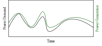
Does it meet demand at all times? Yes. Does it produce too much power? No, which means we spent as little as possible so it was a cheap solution. But what happens if we look at the same day on the previous year?
On the previous year, the demand curve was very similar, yet the solution isn't valid anymore. This is because we optimised for a single sample (curve) and didn't consider any variations.
- \(x\) - How many generators we build, and where, as a binary vector.
- \(p_t\) - How much power a generator builds at a given time \(t\), again as a vector.
- \(d_t\) - How much power demand there is at a given time \(t\), as a scalar.
- \(c\) - How much each generator costs to build, as a vector.
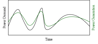
Does it meet demand at all times? Yes. Does it produce too much power? No, which means we spent as little as possible so it was a cheap solution. But what happens if we look at the same day on the previous year?
On the previous year, the demand curve was very similar, yet the solution isn't valid anymore. This is because we optimised for a single sample (curve) and didn't consider any variations.
Better Approaches
If we let \(d\) represent a single demand curve, there are a few ways to deal with this. Firstly, we could look at the samples of many years in the past and use
them to form a probability distribution. Our \(d\) is then the mean of this distribution. We can optimise for this mean - which is called stochastic optimisation.
This is the obvious choice, however interestingly it doesn't work well at all. We could also consider robust optimisation, where
instead of just a single sample you take an entire set \(D\) containing any number of samples (possibly infinite) and aim to find a solution that
works for the worst case (which by definition means any \(d \in D\)).
Robust optimisation is better, but it is quite conservative, usually it will build too many generators preparing for a scenario that will never happen.
Stochastic
$$
\begin{align}
\min_{x} &\quad c^\top x\\
\text{s.t.} &\quad p_t^\top x \geq \mathbb{E}[d_t],\quad d_t \sim D_t,\quad \forall t
\end{align}
$$
Robust
$$
\begin{align}
\min_{x} &\quad c^\top x\\
\text{s.t.} &\quad p_t^\top x \geq d_t,\quad \forall d_t \in D_t,\quad \forall t
\end{align}
$$
Distributionally Robust Optimisation
If stochastic optimisation is too optimistic, and robust optimisation is too pessimistic, the solution must be something in between the two.
This is called distributionally robust optimisation, which is a state-of-the-art technique. We take our empirical distribution we call \(D\) (what we used for stochastic optimisation
made from historical data), and we build a set of all probability distributions which are similar to it - we call this \(\mathcal{A}\). We find a solution that is valid
for the expected value of any possible distribution \(D\) we may choose from \(\mathcal{A}\).
$$
\begin{align}
\min_{x} &\quad c^\top x\\
\text{s.t.} &\quad p_t^\top x \geq \mathbb{E}[d_t],\quad d_t \sim D_t, \quad D_t \in \mathcal{A}_t, \quad \forall t
\end{align}
$$
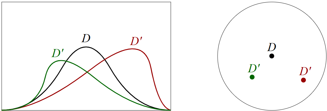
For example, in the image below, we may take demand samples \(d_1, d_2, \ldots\) from previous years to form our empirical distribution \(D\).
Then, distributions which are similar (the red and green \(D'\) distributions), will be included in the ambiguity set \(\mathcal{A}\) (the circle) and we
optimise to find a solution that works for all of them.
More formally, the ambiguity set is not simply a circle drawn around a dot, it is a Wasserstein ball with a radius \(r\) that we choose: $$ \mathcal{A} = \{D'\ |\ W_1(D, D') \leq r\} $$ Where: $$ W_p(D, D') = \inf_{\gamma \in \Gamma(D, D')}\left(\mathbb{E}[f(d, d')^p]\right)^{1/p},\quad (d, d') \sim \gamma $$ This set \(\mathcal{A}\) actually contains an infinite number of distributions, therefore we spent time reformulating it into a solvable form (while still making sure our solution is valid for the whole infinite set!) which allows the optimiser to strike the right balance between cost and reliability.
More formally, the ambiguity set is not simply a circle drawn around a dot, it is a Wasserstein ball with a radius \(r\) that we choose: $$ \mathcal{A} = \{D'\ |\ W_1(D, D') \leq r\} $$ Where: $$ W_p(D, D') = \inf_{\gamma \in \Gamma(D, D')}\left(\mathbb{E}[f(d, d')^p]\right)^{1/p},\quad (d, d') \sim \gamma $$ This set \(\mathcal{A}\) actually contains an infinite number of distributions, therefore we spent time reformulating it into a solvable form (while still making sure our solution is valid for the whole infinite set!) which allows the optimiser to strike the right balance between cost and reliability.
Final Product
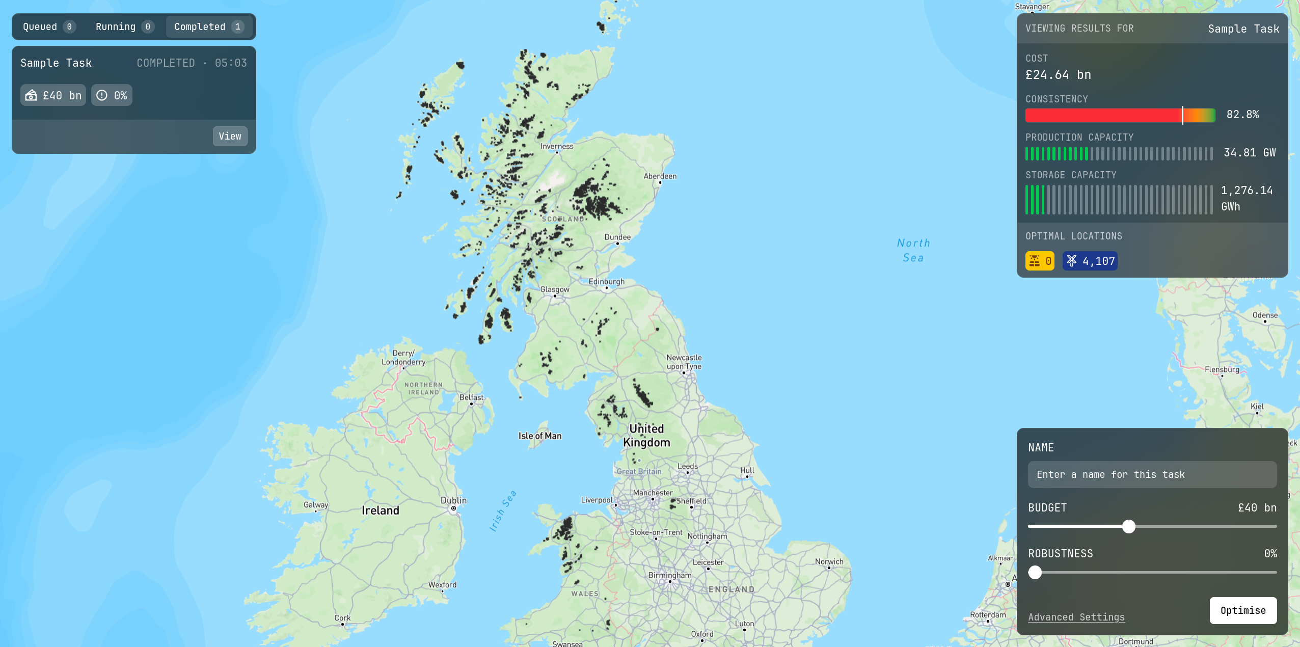
While there was a lot of theory involved, there was also a significant amount of code. A zoomable interative
map was implemented with customisable parameters and a database of past solutions to make it useful for policy makers.
Feedback
- "Excellent. Two-prong methodological approach with LP and DRO formulations aimed at, overall management approach and tools used, extensive testing and study of robustness of solutions produced. Code extendable and modular with identified future directions to integrate additional sources or model based forecasts."
- "Excellent structure, presentation, balance of highly challenging technical material and real-world experimentation and application with back/front end development and impressive demos."